.ipynb .pdf

Binder

Contents

Introduction

In the most general sense, \(\mathrm{dynamics}\) is the study of properties or parameters that evolve or change with respect to some other parameter. For example, the field of population dynamics studies the change of animal or human populations.

In the context of this text and class, we will study the parameters the describe the motion of bodies. More often than not, the changes in these parameters with respect to time will be of interest.

At a physical level, our focus will be on the motion of bodies, which we assume can be categorized under two classes:

1. Particles: These are objects that can be modelled as point masses. They have negligible dimension.

2. Rigid bodies: These objects that have some shape. Also, these objects do not deform when a force is applied to them.

This module could also be called Rigid Body Dynamics. Studying the dynamics involving the motion of particles and bodies has two distinct parts:

1. Kinematics: the study of the geometry or mathematics of motion, without taking into consideration any forces that cause motion. The parameters of interest here are positions, velocities, and accelerations. This is also called rigid body motion or rigid body kinematics.

2. Kinetics: the study of motion while accounting for any forces causing the motion by using Newton’s laws.

Useful fundamental concepts

The following definitions are used in kinematics:

1. Particles: Objects that can be modelled as point masses, having negligible dimension.

2. Point: A massless particle.

3. Rigid bodies: Objects that have some shape. They can have a mass or be massless. Also, these objects do not deform when a force is applied to them.

4. Reference frame: A massless rigid body with respect to which an analyst observes and measures motion of objects.

Pictorial representation

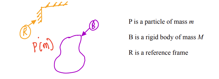
Attention

In rigid body kinematics, we aim to mathematically describe the motion of \(B\) and \(P\) in \(R\).

• This requires pre-requiste knowledge on:
  (i) vectors: unit vector, general vector, component form
  (ii) vector algebra: addition of vectors multiplication of vectors
  (iii) vector calculus: vector differentiation
  

Revision: Vectors Fundamentals

• scalar: A quantity described purely by a number.
        e.g. \(1, 2, 3\ldots\); one pint of beer
  

• vector: a quantity characterised by both magnitude and direction.

• Notation: commonly, written using letters from the English and Greek alphabets.

Representation

Vectors are drawn as a directed line segment (i.e., a line segment with an arrow at one end).

They are typically represented for two cases:

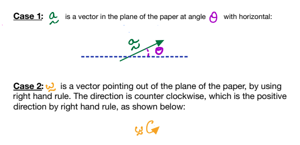
Conversely, by the same rule, a clockwise vector will have a negative direction and points into the plane of the paper. The convention is shown below for a vector \(\vec{\mathcal{L}}\):

Attention

The inclination of clockwise and counterclockwise vectors is \(90^{\circ{}}\) with respect to the plane of the paper.

Unit vector

A vector of unit magnitude (i.e., its magnitude is \(1\)).

Unit vectors are commonly written with a caret \((\widehat{\ })\) over a letter in the alphabet. For example, \(\hat{i}\) is a unit vector and \(\left|\left|\hat{i}\right|\right|=1\) says that magnitude of \(\hat{i}\) is \(1\).

Reference frames

A set of three unit vectors that are mutually orthogonal.

In the figure below, \(X-Y-Z\) form a Cartesian coordinate system. \(\hat{i},\;\hat{j}\;\& \;\hat{k}\) are a set of unit vectors that are mutually orthogonal and directed along \(X-Y-Z\) respectively.

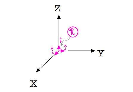
The set of unit vectors are right-handed (also known as a “dextral set”), which means the following relationships hold true:

\[\begin{split} \hat{i} \times \hat{j} = \hat{k} \\ \hat{j} \times \hat{k} = \hat{i} \\ \hat{k} \times \hat{i} = \hat{j} \\ \end{split}\]

The set of unit vector form a reference frame \(R\).

Reference frames are useful for studying moving objects. This will become apparent in the coming weeks of lectures.

An alternate notation for unit vectors that make up a reference frame commonly used for dynamics is shown in the figure below; it makes use of subscripts in \(x\), \(y\), and \(z\) directions to make it explicit along which coordinate axis the unit vectors are aligned. We will (almost always) see (and use) such subscript-based notations in these notes for sake of clarity.

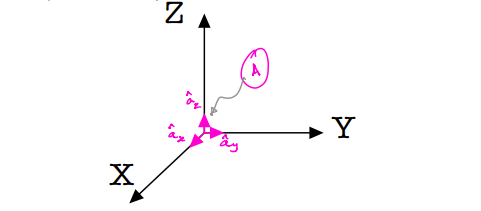
• \(\hat{a}_x\) is the unit vector along the \(X\)-direction

• \(\hat{a}_y\) is the unit vector along the \(Y\)-direction

• \(\hat{a}_z\) is the unit vector along the \(Z\)-direction

This is a dextral set of unit vectors, which form a reference frame \(A\).

\[\begin{split} \begin{align} \hat{a}_x \times \hat{a}_y =& \hat{a}_z \\ \hat{a}_y \times \hat{a}_z =& \hat{a}_x \\ \hat{a}_z \times \hat{a}_x =& \hat{a}_y \\ \hat{a}_x \times \hat{a}_z =& -\hat{a}_y \\ \hat{a}_z \times \hat{a}_y =& -\hat{a}_x \\ \hat{a}_y \times \hat{a}_x =& -\hat{a}_z \\ \end{align} \end{split}\]

Component form

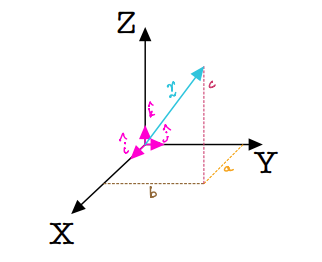
In the figure below, \(\vec{r}\) is a vector with coordinates \(a,\;b,\;c\) in \(X-Y-Z\), respectively.

Note

\(a,\;b,\;c\) are scalars.

The component form of \(\vec{r}\) is given by:

\[ \vec{r} = a\hat{i} + b\hat{j} + c\hat{k} \]

This is the “component form” of expressing vectors, which makes use of scalars and unit vectors.

Vector algebra using a CAS (Computer Algebra Systems)

Attention

Please review addition and multiplication of vectors.

In this module on dynamics, we will exploit a computer algebra system (CAS, for short) to perform some key vector algebra operations. A CAS is a software that allows manipulation of non-numerical as well as numerical mathematical expressions in a manner similar to that done manually, by humans.

SymPy is a free CAS that we will use in studying dynamics. It has many advanced features that are particularly useful in studying rigid body dynamics.

This set of notes is accompanied by an “interactive textbook” that you can utilise on a web browser; this is enabled by Porject Jupyter.

The textbook has activities that are to be performed on JupyterLab; these activities have the Jupyter icon next to them:

• Written content: This similar to any textbook. The textbook style portion is rendered on the browser.

• Code cells: Within this one performs relevant computations by writing “lines of code”. When using the JupyterLab interface, you can type click within the code cell to enter some text.

Warning

Your coursework will be assigned on this platform by instructors. You will complete and submit all your coursework here.

Please proceed to this notebook to review vector algebra.

Vectors and Reference Frames

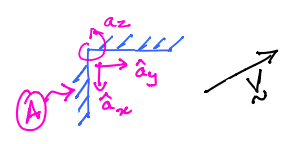
• The figure above shows a reference frame \(A\) and vector \(\vec{v}\).

• \(\vec{v}\) is said to be fixed in the frame \(A\) if and only if none of the characteristics of \(\vec{v}\) are seen to change when it is observed from \(A\).

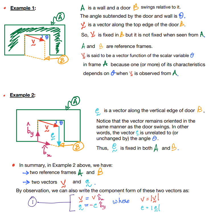
Notice that I have introduced the unit vectors \(\hat{b}_x\) and \(\hat{b}_y\) for the reference frame \(B\) but \(\hat{b}_z\) is not shown though it is orthogonal to both \(\hat{b}_x\) and \(\hat{b}_y\).

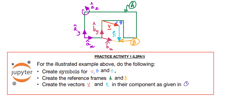
For sake of developing subsequent discussions, we will now also introduce a dextral set of unit vectors for frame

\[ A: \: \hat{a}_x,\;\hat{a}_y\:\&\:\hat{a}_z \]

Rigid Body Kinematics: Orientations

Kinematics or Rigid body kinematics is the study of motion while ignoring the cause of motion.

In kinematics, we are interested in “position”, “velocity”, and “acceleration” and the relationship between them.

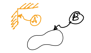
In other words, using the figure below, we are interested in describing the motion of \(B\) in \(A\).

Classification of Rigid Body Motion

Translation: the motion of \(B\) in \(A\) is a translation if and only if any straight line segment embedded in \(B\) remains parallel to itself when observed from \(A\) when \(B\) moves in \(A\). If this condition is not met, then we have to consider the motion as rotation.

Simple rotation: the motion of \(B\) in \(A\) is a simple rotation if and only if there exists a unit vector \(\hat{n}\) that remains fined in both \(B\) and \(A\), as \(B\) moves in \(A\). Examples in figures below:

Coming back to our old example of a door hinged to a wall.

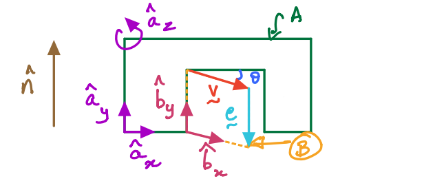
Here, \(\hat{b}_y\) is a unit vector that is fixed in both \(B\) and \(A\). Using our definition for simple rotation tells us that \(\hat{b}_y\) is \(\hat{n}\). So, in mathematical notation, we can say:

But we must now pause to ask ourselves if there is any other unit vector that is also fixed in both \(B\) and \(A\)? It turns out that there is, indeed, another one fixed in both \(B\) and \(A\): \(\hat{a}\).

So we can now also write:

So, from \(2\) and \(3\), we get:

Why is establishing \(4\) useful and critical?

So far, we have written the vectors \(\vec{v}\) and \(\vec{e}\), in terms of the \(B\) frame. As a result, they were not functions of \(\theta\).

Expressing the vectors in the unit vectors attached to the A frame requires us to derive relationships between \(\hat{a}_i\) and \(\hat{b}_i\):

\[ <i = x,y,z> \]

\(4\) allows us to derive a relationship between \(\hat{a}_i\) and \(\hat{b}_i\), which then provides a basis for developing the rigid body kinematics.

Let us explore how to derive these relationships for the vectors \(\vec{e}\) and \(\vec{v}\) in the doorwall example (figure is shown again below):

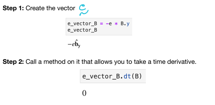
From the second of Equations in \(1\), we have \(\vec{e} = -e\hat{b}_y\).

From \(4\) we also get \(\vec{e} = -e\hat{a}_y \:\:\:(5)\)

\(\theta \)in the prior example is an angle that describes the orientation of \(B\) relative to \(A\) (and vice versa). Thus, it is also called an angular position. Other common ways of referring to it are orientation angle or attitude angle.

Now, we come to a more involved example, where we will express \(\vec{v}\) in terms of the unit vectors of the \(A\) frame using the first of Equations \(1\) as the starting point:

\[ \vec{v} = v\hat{b}_x \]

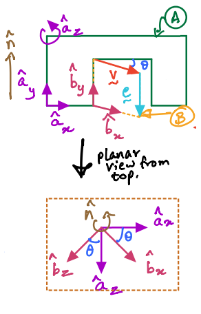
We can now examine the relationships between the unit vectors by drawing only the unit vectors with the vector \(\hat{n}\) out of the plane (see figure below this passage). We can then derive the following relationships by examining the lower figure, comprising only unit vectors:

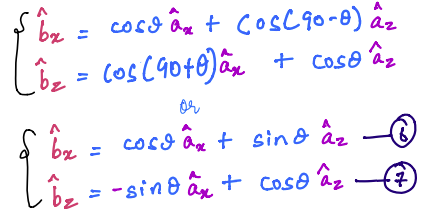
Therefore from \(6\):

\[ \vec{v} = v(\cos{\theta}\hat{a}_x + \sin{\theta}\hat{a}_z) \]

Also from \(5\), we have: \(\hat{b}_y=\hat{a}_y\)

Now, we have derived the complete relationships between the unit vectors that make up the \(B\) frame in terms of the unit vectors of the \(A\) frame.

We can take this work one step further and write the relationships in matrix form as follows:

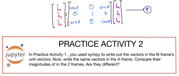
Let’s focus on the second row of the above matrix equation (this is highlighted in yellow below):

This tells us that: \(\hat{b}_y=\hat{a}_y\)

Visually, this can be interpreted to mean that the door B swings relative to the wall \(A\) about the \(\hat{b}_y\)-axis, which also coincides with the \(\hat{a}_y\)-axis. In other words, this represents what is know a simple rotation about the \(y\)-axis. Similar relationships can also be derived for simple rotations about \(x\)-axis or \(z\)-axis.

Direction Cosine Matrix (DCM)

Continuing with the matrix representation of the door-wall example, the \(3\times3\) matrix (highlighted in green above) relates the \(B\)-frame’s unit vectors to the \(A\)-frame’s unit vectors. It is called the direction \(\text{cosine}\) matrix of \(A\) in \(B\). The symbolic notation of it is \({}^{B}C^{A}\). This is for a rotation about \(y\)-axis, as mentioned on the previous page.

Simple notations about \(z\)-axis would result in the following DCM.

Simple notations about \(x\)-axis would result in the following DCM:

Why does the term DCM have \(\text{cosine}\) in it?

Return to Equations \(6\) and \(7\), you can observe that they were derived purely using the \(\text{cosine}\) of angles between different unit vectors. For example, consider the \(x\)-unit vector of the \(B\)-frame as represented in the \(A\)-frame:

\[ \hat{b}_x = \cos{\theta}\hat{a}_x + \cos{(90-0)}\hat{a}_z \]

which then becomes

\[ \hat{b}_x = \cos{\theta}\hat{a}_x + \sin{\theta}\hat{a}_z \]

This can be written in a more generic form using only dot products (as this product is defined using \(\text{cosine}\) terms), as shown below:

\[ \hat{b}_x = (\hat{b}_x\cdot{}\hat{a}_x)\hat{a}_x + (\hat{b}_x\cdot{}\hat{a}_y)\hat{a}_y + (\hat{b}_x\cdot{}\hat{a}_z)\hat{a}_z \]

where,

\[ \hat{b}_x\cdot{}\hat{a}_y \Longrightarrow \cos{90^{\circ}} = 0 \]

This serves as the foundation for a more general description of orientations for General \(3D\) Rotation.

General \(3D\) Rotation and DCM

Below, body \(B\) is moving freely relative To frame \(A\):

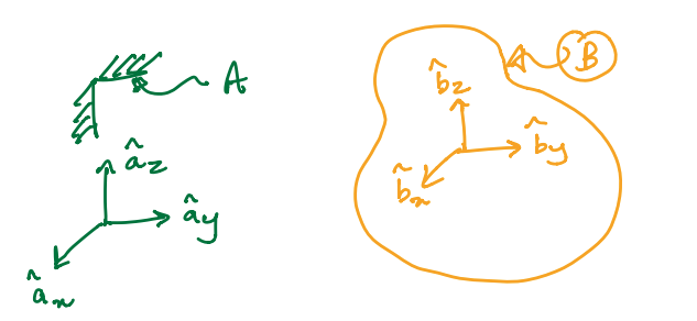
From the preceding discussion on dot products and DCM, we can write the following relationships between two reference frame \(A\) and \(B\).

\(11\) can then also be written in the matrix form as shown below:

which can also be written more succinctly as:

\({}^{B}C^{A}\) is the direction \(\text{cosine}\) matrix of \(B\) and \(A\).

Note

\({}^{A}C^{B} \neq {}^{B}C^{A}\)

A key property of DCM

A very important property of DCM is that it is an orthogonal matrix. Mathematically, this means that the inverse of the DCM is the same as the transpose of the matrix. In other words, if the DCM is given by a matrix \(M\), then:

This is a very useful result because it is considerably easier to compute the transpose of a matrix than it is to compute its inverse.

How is this property useful?:

At this point, we two that we can express the same vector in different reference frames. This property allows us to do so in a very easy manner. Below we show how you can easily convert (or express) a vector given in the \(B\)-frame to its equivalent in the \(A\)-frame.

In fact, when one compares \(15\) to \(8a\) one sees that:

\[ {}^{B}C^{A} = {\left({}^{B}C^{A}\right)}^T \]

Vector Calculus

The area of calculus we are concerned with is the time derivatives of vectors which result in velocities and accelerations.

In the case of vector, it is critical to consider the reference frame when computing derivatives. This is not the case for scalars.

Caution

Computing the time derivative from frame \(A\) of any arbitrary vector \(\vec{x}\), we must express the vector in unit vectors attached.

If the component form of \(\vec{x}\) is given in the frame \(A\) by:

\[ \vec{x} = x_1\hat{a}_x + x_2\hat{y}_x + x_3\hat{a}_x \]

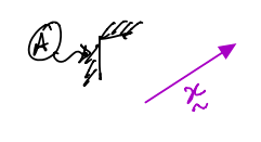
then

\[ \frac{{}^{A}d\vec{x}}{d\theta} \triangleq \left(\frac{d\hat{x_1}}{d\theta}\right)\hat{a}_x + \left(\frac{d\hat{x_2}}{d\theta}\right)\hat{a}_y + \left(\frac{d\hat{x_3}}{d\theta}\right)\hat{a}_z \]

Doorwall example

Notation:

\[\begin{split} \frac{{}^{A}d\vec{e}}{dt} = \text{is the time derivative of the vector } \vec{e} \text{ when observed from the }\\ \text{reference frame } A\text{. So, } \vec{e}= h\hat{b}_y = h\hat{a}_y \end{split}\]

Therefore,

\[ \frac{{}^{A}d\vec{e}}{dt} = \frac{{}^{A}d(h\hat{a}_y)}{dt} = 0 \text{ (zero vector)} \]

So, how can we compute the derivative of a vector using SymPy?

Another example:

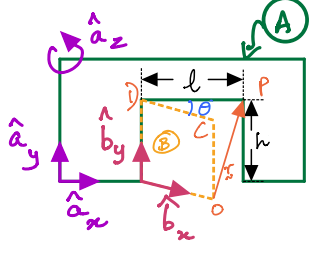
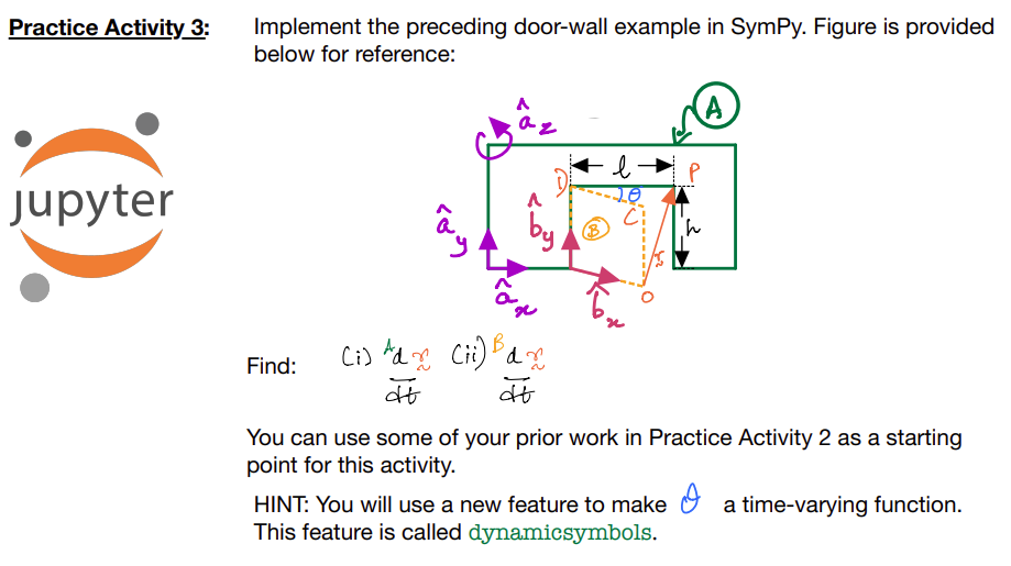
\(O\), \(C\), \(D\) and \(P\) are points as shown in the figure. \(l\) and \(h\) are the length and height of the door. \(\theta\) is timevarying. You are asked to find (i.e., compute symbolic expressions) for the following:

All final answers are to be expressed in unit vectors attached to the \(A\)-frame.

Solution

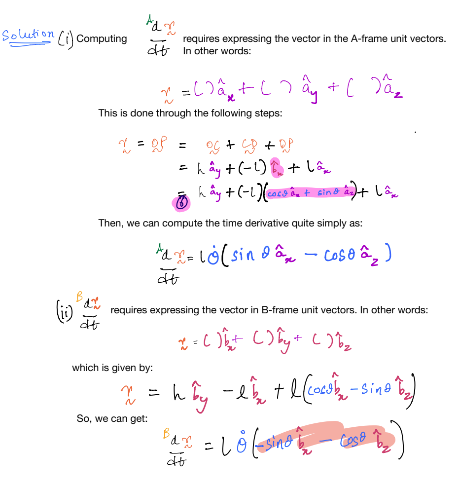
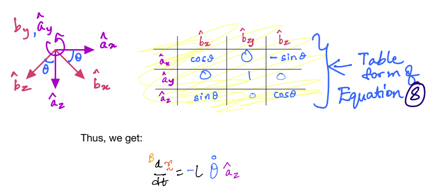
The above example demonstrated the difference between taking time derivatives of the same vector from two frames.

Properties of Vector Derivatives

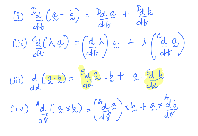
where,

• \(\vec{a},\;\vec{b},\;\vec{c}\) are arbitrary vectors.

• \(\theta,\;\lambda,\;\alpha,\;\gamma\) are scalars.

• \(t\) is scalar time.

Rigid Body Kinematics: Angular Velocity and Angular Acceleration

Angular velocity:

Angular velocity is defined as the time rate of change of orientation.

Angular velocity is denoted using the greek letter omega. For example, in the figure below, \({}^{A}\vec{w}^{B}\) is the angular velocity of B in A

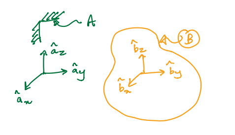
Case 1: Simple Rotation

The motion of \(B\) in \(A\) is a simple rotation if and only if there exists a unit vector \(\hat{n}\) that remains fixed in both \(B\) and \(A\) as \(B\) moves in \(A\). Mathematically, simple rotation leads to

Examples

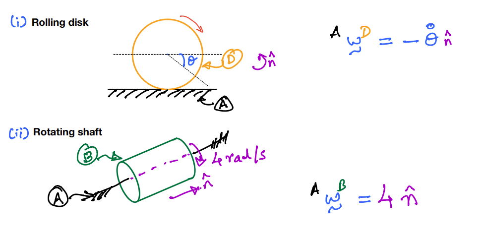
Case 2: General 3-D Rotation

Below, body \(B\) is moving freely relative to frame \(A\).

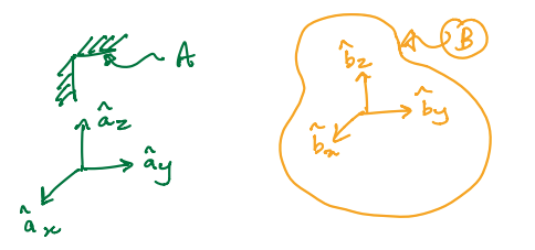
\(\hat{b}_x\), \(\hat{b}_y\) and \(\hat{b}_z\) are rigidly fixed to \(B\).

The angular velocity of body \(B\) in frame \(A\) is mathematically defined as:

which can then be written in a more compressed form as:

where \(w_x,\;,w_y,\;w_z\) are scalar components of the angular velocity vector in the \(x\), \(y\), and \(z\) directions respectively.

Chain rule for angular velocity

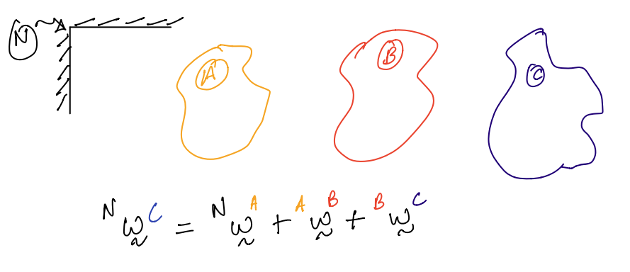
Angular acceleration:

Angular acceleration is the time rate of change of angular velocity vector.

In the figure above, \(B\) is moving freely in \(A\). The angular acceleration of \(B\) in \(A\) is denoted as \({}^{A}\vec{\mathcal{L}}^{B}\)

It is defined as:

\[ {}^{A}\vec{\mathcal{L}}^{B} = \frac{{}^{A}d}{dt}{}^{A}\vec{w}^{B} \]

Indeed, one must be careful to express the angular velocity in the appropriate reference frame prior to computing its time derivative. Unfortunately, it is not always convenient (or desirable and might even be impossible) to switch between reference frames before computing the derivative. So, some special results are presented to tackle such scenarios, which are presented after the next example.

Example

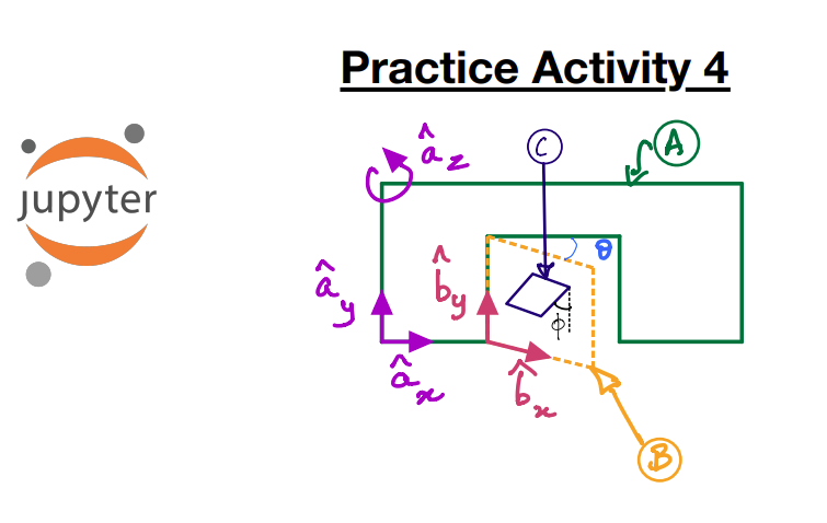
The door-wall example is modified to have an additional object: a cat flap \(C\) which makes an angle \(\phi\) with the door’s \(y\)-axis.

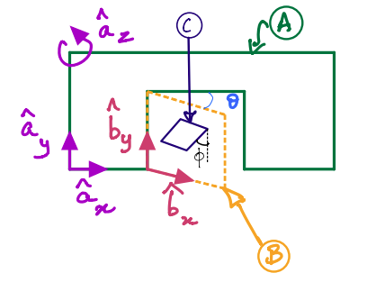
You are asked to compute the angular acceleration of the cat flap \(C\) with respect to \(A\).

Solution

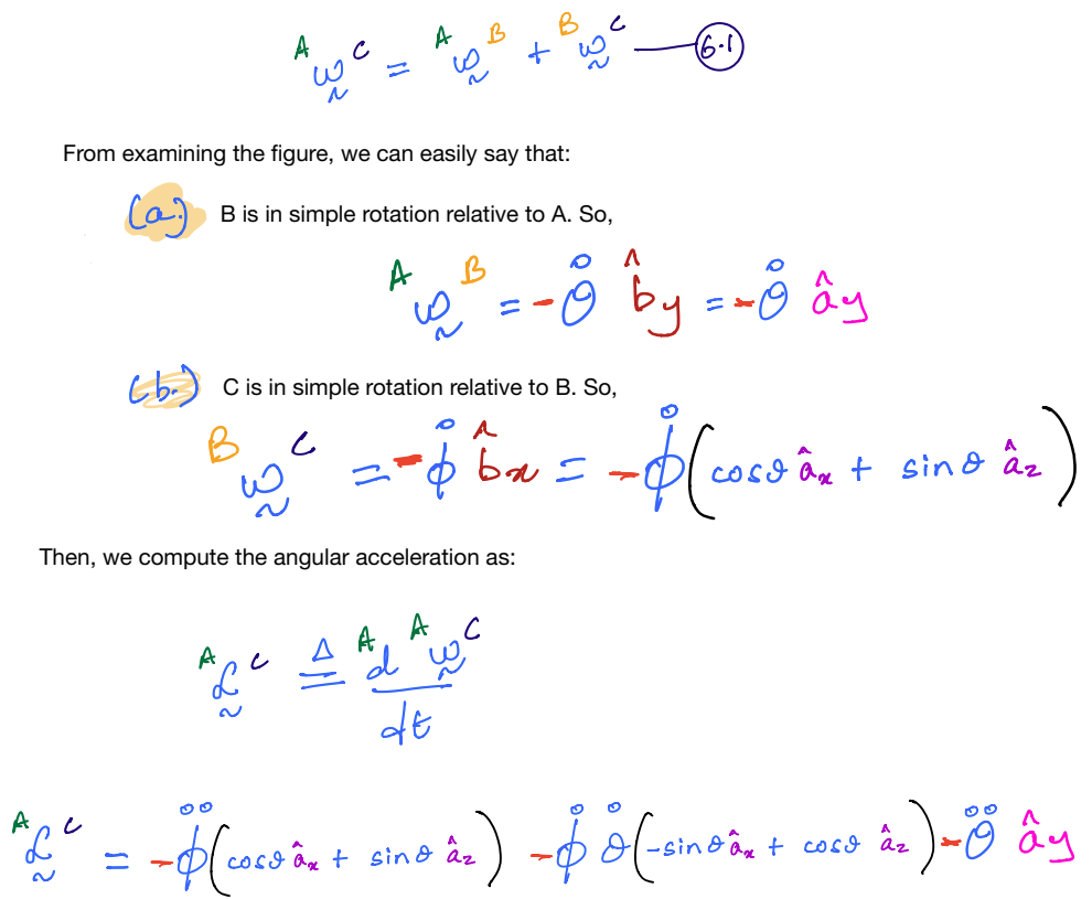
Special results involving time derivatives

KEY RESULT 1

As before, \(A\) is a fixed reference frame with unit vectors rigidly attached to it, i.e., \(\hat{a}_i(i=x,y,z)\).

Likewise, \(B\) is a rigid body with unit vectors rigidly attached to it, i.e., \(\hat{b}_i(i=x,y,z)\).

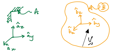
\(\vec{v}\) is an arbitrary vector that is fixed in \(B\) and given in its component form by:

\(v_1, v_2, v_3\) are the scalar components of \(\vec{v}\) in frame \(B\) and as it is fixed in \(B\) it follows:

Example

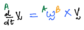
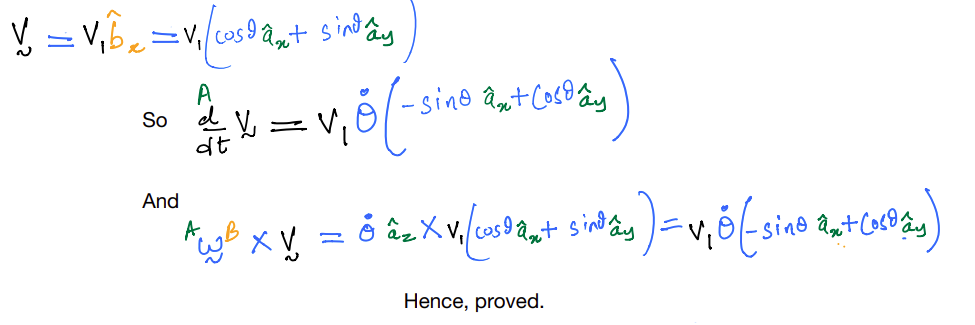
We will prove key result 1 (boxed in red above) is true for a trivial case: simple rotation.

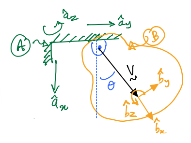
As before, \(A\) is a fixed reference frame with unit vectors rigidly attached to it, i.e., \(\hat{a}_i(i=x,y,z)\).

Likewise, \(B\) is a rigid body with unit vectors rigidly attached to it, i.e., \(\hat{b}_i(i=x,y,z)\).

\(B\) is hinged to \(A\) such that it is in simple rotation, such that:

\(\vec{v}\) is an arbitrary vector that is fixed in \(B\) and given in its component form by: \(\vec{v}=v_1\hat{b}_x\)

Prove that:

Solution

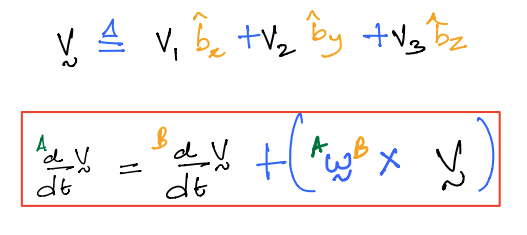
KEY RESULT 2

As before, \(A\) is a fixed reference frame with unit vectors rigidly attached to it, i.e., \(\hat{a}_i(i=x,y,z)\).

Likewise, \(B\) is a rigid body with unit vectors rigidly attached to it, i.e., \(\hat{b}_i(i=x,y,z)\).

\(\vec{v}\) is an arbitrary vector that is moves relative to both \(A\) and \(B\). It is in its component form by:

Proof

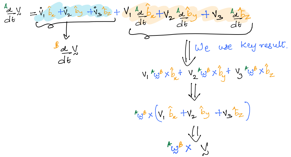
This is a very powerful formula. However, it relies on our ability to derive an expression for the angular velocity vector in an appropriate frame. We will now use it in our cat flap example.

Example

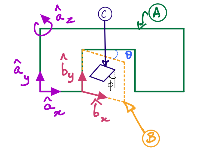
You are asked to find angular acceleration of the cat flap \(C\) with respect to \(A\) using key result 2.

Solution

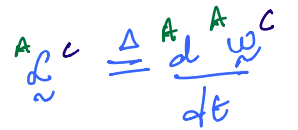
we may then invoke KEY RESULT 2 to rewrite the right hand-side as

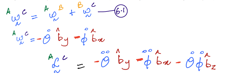
This angular velocity of \(C\) in \(A\) can be computed using the chain rule given by Equation \(6.1\) as:

Particle Kinematics: Position, Velocity, Acceleration

So far, we have analyzed changes in orientations of reference frames and the resulting parameters of angular velocity and angular acceleration. In other words, these parameters measure the changes in angles (or angular positions). Now, we will study changes in positions of points. This topic is also called translational kinematics. A pictorial representation of the problem is shown and then described below.

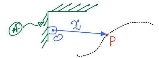
\(O\) is a point rigidly attached to the reference frame \(A\).

\(P\) is a particle of mass \(m\) and is moving along the dashed path. It is said to be translating relative to frame \(A\).

Position of P in A:

We utilize \(\vec{r}\) a position vector to locate \(P\)-the vector has its tail fixed in \(A\) and its tip (or head) tracks \(P\).

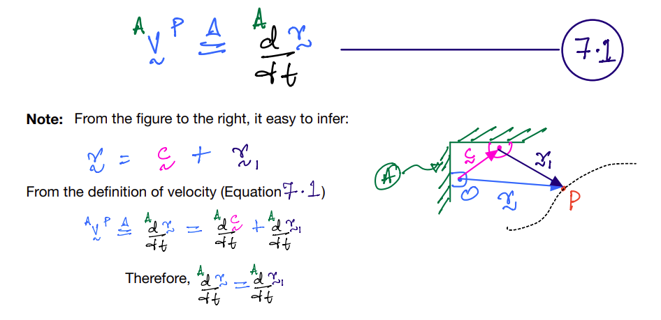
Velocity of P in A:

Notation:

\[ {}^{A}\vec{v}^{P} \]

Mathematically, this velocity of P in A is defined as:

Acceleration of P in A:

Notation:

\[ {}^{A}\vec{a}^{P} \]

Mathematically, this acceleration of \(P\) in \(A\) is defined as:

Example

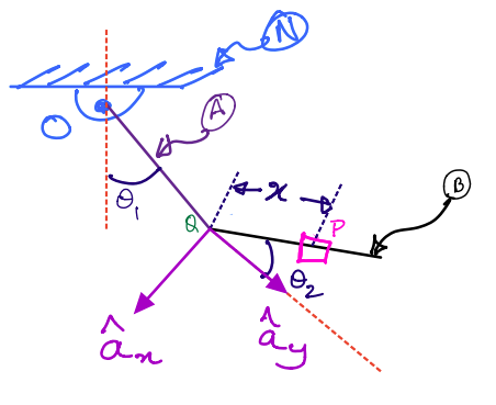
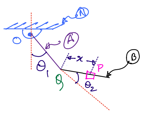
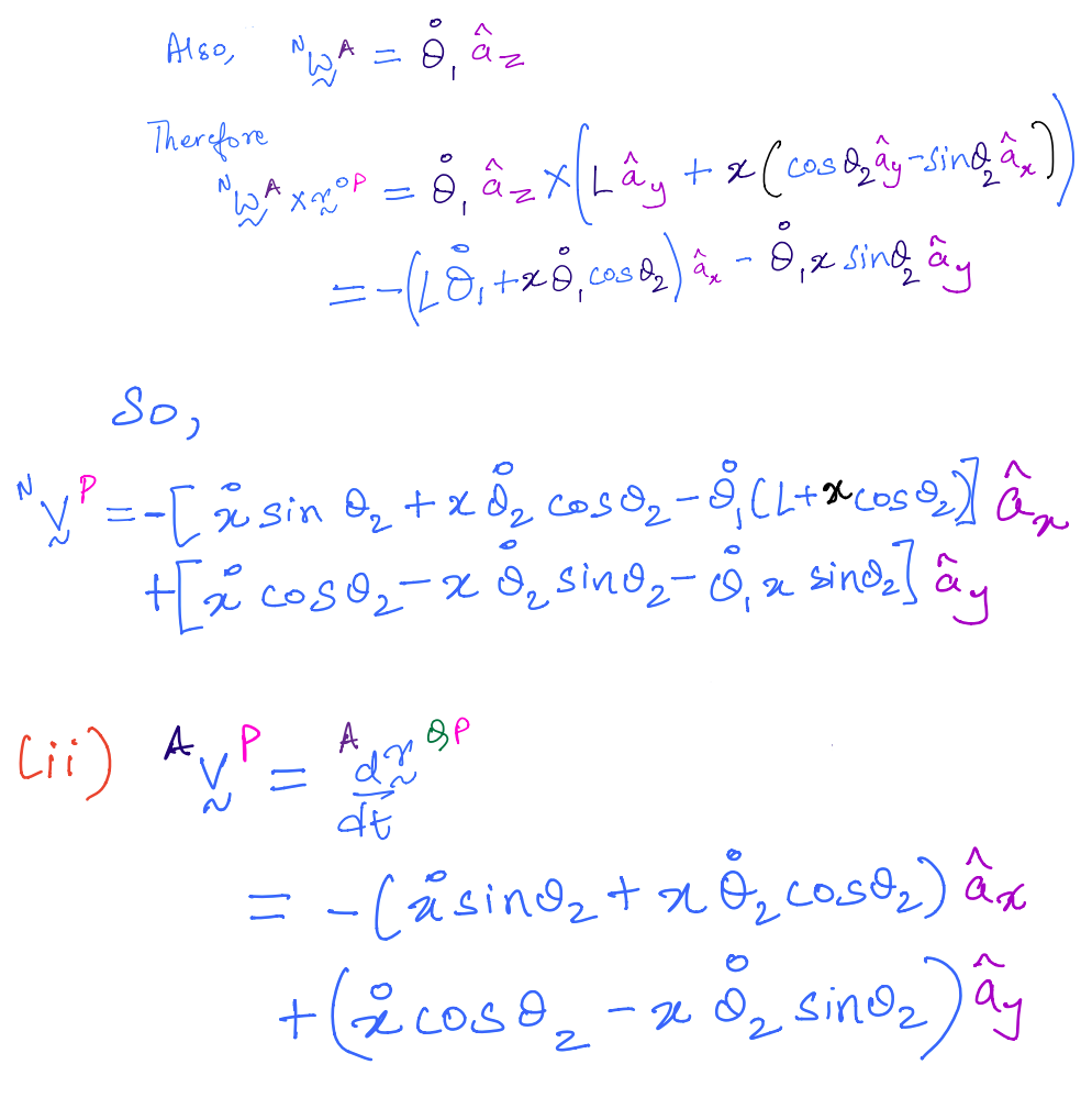
\(N\) is a fixed reference frame to which link \(A\) is attached at a point \(O\). \(B\) is a second link attached to \(A\) at point \(Q\). This system is commonly called a double pendulum. We assume that both links are of the same length \(l\).

\(P\) is a particle that is sliding on \(B\), the second link of the double pendulum. It is located from point \(Q\) by a scalar time-varying parameter \(x\).

The two angles that describe the double pendulum’s two links are also shown in the figure, namely: \(\theta_1\) and \(\theta_2\). You are to compute:

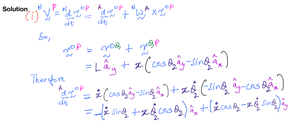
Solution

Two key velocity/acceleration transfer theorems

There are two theorems that are useful in particle kinematics that allow us to compute velocities and accelerations by transferring them to another point. They are discussed below.

Theorem 1: Two-point theorem

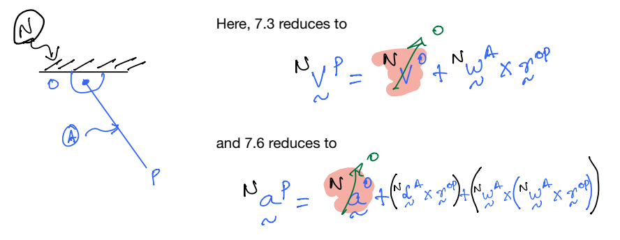
This theorem is useful for determining the velocity (and/or acceleration) of one point on a rigid body by using (or transferring to) another point on the same rigid body.

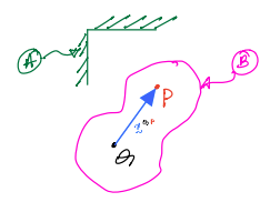
In the above figure, \(P\) and \(Q\) are two points that are rigidly fixed to the same rigid body, \(B\). Further, \(B\) is in freemotion relative to \(A\). In other words, \(B\) is moving freely in \(A\); in other words, it is rotating and translating when viewed from \(A\).

In such a scenario, the following two relationships can be used to compute the velocity and acceleration of \(P\) in \(A\).

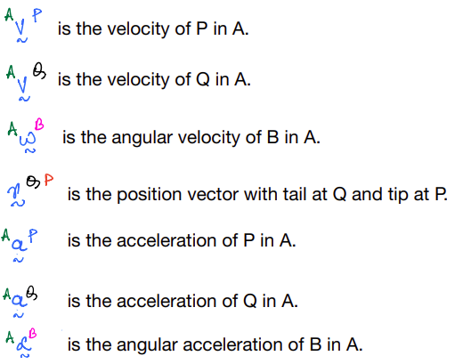
where,

Some special cases of theorem 1

Case 1

If B is purely in translation:

Case 2

If B is in simple rotation about a fixed axis. E.g., a simple pendulum, (see figure).

Case 3

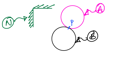
Consider the case shown in the above figure containing two discs, \(A\) and \(B\). The two discs are rolling on each other and maintain a single point of contact \(P\). Their motion is observed from a fixed frame \(N\).

As the point \(P\) is clearly shared between the 2 bodies, we introduce the following notation:

• \(P_A\) is the contact point belonging to body \(A\).

• \(P_B\) is the contact point belonging to body \(B\).

If it is said that A rolls without slip on B, then the following assumption can be made in tackling a problem:

Common example for rolling without slip

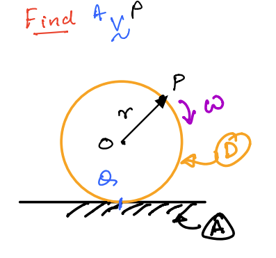
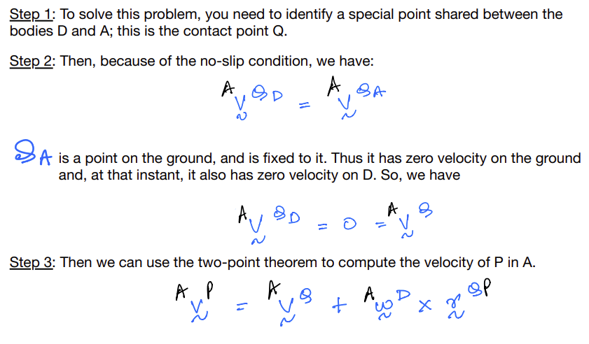
In the figure above, the disk \(D\) rolls without slip on \(A\). \(P\) is a point on the disk’s circumference.

Solution

Theorem 2: One-point theorem

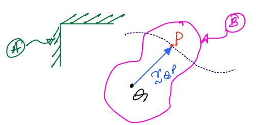
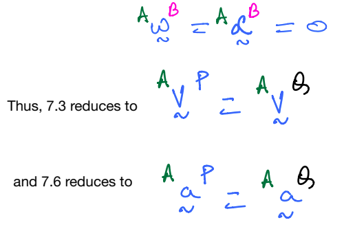
In the above figure, \(P\) is a point that translates relative to body, \(B\). Point \(Q\) is rigidly attached to \(B\). The one-point theorem allows computation of the velocity and acceleration of \(P\) relative to the frame \(A\), while accounting for the relative motion of \(P\) as seen from \(B\). The velocity formula is given by Equation \(7.5\).

\({}^{B}\vec{v}^{P}\) is the velocity of \(P\) in \(B\). This term is also called relative velocity.

The highlighted term is referred to as coincident point velocity. This highlighted set of terms are identical in form to that seen in the two-point theorem.

The acceleration in this scenario is computed from Equation \(7.6\) (also called five-term beast):

The terms in the acceleration equation have special terminology; these are shown below. Also, note that the ‘transport acceleration’ term below is identical in form to the two-point theorem acceleration formula.

Student Activities

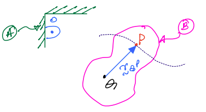
1. Derive relationships \(7.3\) and \(7.4\). You need to make use of key result \(2\) (derivative theorem) and the definitions of velocities and accelerations.

2. Derive the relationships given by and using the figure below. You will need to draw TWO more position vectors for the derivation. In the figure, \(O\) is rigidly attached To \(A\); \(Q\) is rigidly attached to \(B\); \(P\) moves along a path on \(B\); and \(B\) moves freely relative to \(A\).

3. Prove that if \(P\) were rigidly fixed to \(B\), then the onepoint theorem relations result in the the two-point theorem relationships.

4. Find: \({}^{N}\vec{v}^{P}\) and \({}^{A}\vec{v}^{P}\) for the particle sliding on the double pendulum using the relevant velocity transfer theorems, as appropriate.

next

Mass/Inertia Scalars